Introduction
Jump Diffusion Markov Chain Monte Carlo is a combination of MCMC (Markov Chain Monte Carlo) and JD (Jump Diffusion). JD relies upon random jumps, which in this particular computer vision case means deciding to either add or remove the number of elements undergoing diffusion. With each iteration of the program one of three options is selected: no jump, where MCMC progresses as normal; jump up, where another element is added; and jump down, where an element is removed. The particular mode of MCMC used in my program is Gibbs Sampling and will be discussed in detail in the following section.
Gibbs Sampling
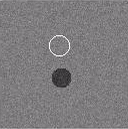
Gibbs Sampling can be easily visualized by the example below: the algorithm executes a random walk in which a random position between a set distance from the given point is chosen and is then evaluated for the probability that it is closer to the object being sought than the current estimate. If the new estimate is determined to be closer to the target object, then the point will move. This action corresponds to the movement of the circle within the example.
Here is a brief explanation of the implementation. The mathematical approach can be seen here.
- Choose a random position within the image as the initial value.
- Take a new sample within five object's width (the object being the circle) of the current sample. Evaluate the new point against the probability distribution and change the location of the point if its probability is greater than that of the previous sample.
- Repeat X times (100 in this case).
Simultaneous Sampling
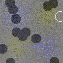
The approach to having an algorithm detect the location of multiple objects seems obvious: simply evaluate the same number of points as there are objects within the image. This line of thinking has two crucial flaws. It doesn't prevent the points from converging to the same object, and it doesn't account for the possibility that the algorithm might not always know how many objects there are in a particular image. I initially approached the problem while ignoring the object quantity issue by telling the algorithm how many objects are within the image and focusing on preventing multiple instances of Gibbs Sampling from locating the same point.
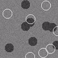
My algorithm creates a small deadzone around each sample that is above a certain likelihood to be positioned over an object, such that the rest of the samples cannot converge to the same point. A crude implementation of this algorithm can be visualized above.
Full JDMCMC
Below is a working example in which single sample expands to twelve, all of which are independently going about Gibbs Sampling. Multiple samples are quickly added to the initial one as the algorithm determines that there exist other high probability locations in addition to those of the existing sample(s). This process works in reverse as well. For example, if thirty samples are used on the same image below that contains only twelve, then the algorithm will eventually reduce the total quantity of samples down to twelve as it determines that the highest numbered sample is of particularly low probability of being in proximity to an object with each iteration.